Lab 3: Inverse Kinematics and Trajectory Tracking
Goal
Implement inverse kinematics for a robot leg and create a trajectory tracking system using ROS2.
Lab Review Slides: Lab 3 slides
Please also fill out the lab document .
Part 0: Setup
Build remaining legs for Pupper. Follow the build instructions to assemble the last legs of Pupper, keeping note that all the pieces for each leg are correctly labeled (each right leg piece has an R on it, and each left leg piece has an L on it).
Open the lab 3 code repository (lab 3 code repository) on your GitHub account. Then, fork the repository to your own GitHub account following the instructions in 🍴 Forking Repositories Guide.
Open the lab 3 folder in VSCode
cd ~/lab_3_fall_2025
code .
Examine
lab_3.pyto understand the structure of theInverseKinematicsclass and its methods.
Part 1: Forward Kinematics on Right Front Leg
Open
lab_3.pyand locate theforward_kinematicsmethod in theInverseKinematicsclass.In this lab, we will instead use the right front leg of Pupper. Implement the
forward_kinematicsmethod for the right front leg. This should be very similar to your implementation of the front left leg from lab 2. You can refer to the lab_2_slides for the fk transformations on the right leg.
Part 2: Implement Inverse Kinematics
Find the
inverse_kinematicsmethod in theInverseKinematicsclass.
TODO 1: Implement the cost_function(theta) for inverse kinematics. This function returns cost, a scalar, and l1, a vector of size 3.
Use the
forward_kinematicsmethod to get the current end-effector position.Calculate the L1 distance between the current and target end-effector positions.
Return the sum of squared L1 distances as the cost (AKA the squared L2 norm of the error vector).
TODO 2: Implement the gradient(theta, epsilon) function to calculate the numerical gradient for inverse kinematics.
Note
Understanding Numerical Gradient Calculation
For numerical gradient calculation, we use the finite difference method to approximate the gradient of the cost function with respect to each joint angle. For a joint angle θᵢ, we calculate:
where:
C(θ) is the cost function (squared L2 norm of end-effector position error)
ε is a small value (e.g., 1e-3)
θᵢ is the i-th joint angle
TODO 3: Implement the gradient descent algorithm for inverse kinematics.
Define the learning rate, maximum number of iterations, and tolerance as hyperparameters. We recommend starting with a relatively large learning rate (e.g., 5), which is higher than what is typically used when training neural networks. Tolerance is measured in meters.
Update the joint angles using the calculated gradient.
Stop the iteration if the mean L1 distance is below the tolerance.
Bonus: Implement a quasi-Newton’s method for faster convergence. Check out the BFGS method if you’re feeling ambitious. This method estimates the inverse Hessian matrix using the gradient and the previous iterations.
DELIVERABLE: We use squared L2 norm for our cost function (AKA objective function or loss function). Why is this a useful objective? Why not use L1?
DELIVERABLE: What happens if the learning rate is too small… what if the learning rate gets too big? (Note: for Pupper’s safety, don’t change the learning rate in the code)
DELIVERABLE: We are using a numerical differentiation approach to calculate the gradient of the cost function. However, this cost function is fairly simple and the gradient could be computed analytically (we use finite differentiation due to simplicity). Think about different loss functions. Where would a numerical gradient come in handy, and where would an analytical gradient be better?
Part 3: Implement Trajectory Generation
Locate the
interpolate_trianglemethod in theInverseKinematicsclass.
TODO 4: Implement the interpolation for the triangular trajectory.
You need to create a function that performs linear interpolation between the triangle’s vertices. The trajectory should loop smoothly from vertex 1 to 2, vertex 2 to 3, and then from vertex 3 back to vertex 1 based on the time variable. The input to the function is a time variable t that dictates where along the triangle’s edges the point currently lies for a given 3-second period. Each vertex transition (e.g., from vertex 1 to vertex 2) should last approximately 1 second. For example, 0 <= t < 1 should interpolate between vertex 1 and vertex 2.
Use the provided
ee_triangle_positions, which define the 3 vertices of the triangle trajectory (this is a 3x3 matrix).Implement linear interpolation between the triangle vertices based on the input time
t. You can use thenp.interpfunction from NumPy to handle the interpolation, or write your own weighted sum function to achieve the same effect.Ensure the trajectory loops every ~3 seconds approximately.
DELIVERABLE: This interpolation between the 3 points on a triangle is called the “Raibert Heuristic”, named after the founder of Boston Dynamics. How would you coordinate the movement of 4 legs on a quadruped to make it walk forward, assuming they each follow the Raibert heuristic? Specifically, which legs should be synchronized (same point of the triangle at the same time)? Feel free to draw a diagram.
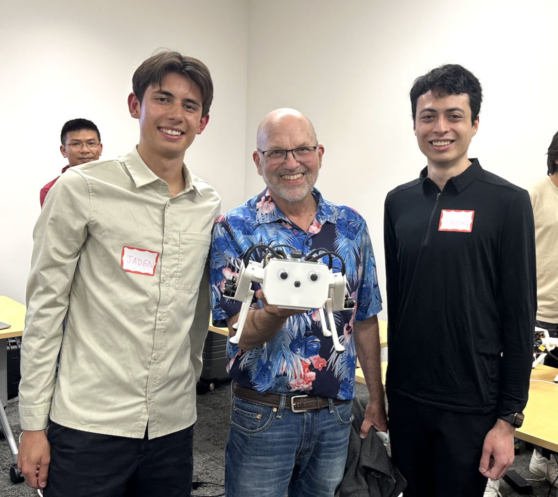
Marc Raibert at the Spring 2023 Pupper demo day.
Part 4: Run and Test Your Implementation
Run the launch file using the following command in
~/lab_3_fall_2025:ros2 launch lab_3.launch.py
On a separate terminal, run the following command to run the
lab_3.pyfile in~/lab_3_fall_2025:python3 lab_3.pyObserve the robot leg’s movement and the terminal output.
Experiment with different trajectory shapes by modifying the
ee_triangle_positionsin the__init__method. If you have recorded the end-effector positions from lab 2, you can use them to set theee_triangle_positionsto match the recorded positions and replay the recorded trajectory!
DELIVERABLE: Take a video of the robot leg tracking the triangular trajectory and submit it with your submission. The triangle motion should be smooth and continuous based on your implementation.
DELIVERABLE: Review question: Why do we need the damping term in PD control? What will happen if damping is too high? Too low?
Part 5: Analyze and Improve Performance
Modify the
ik_timer_periodandpd_timer_periodto see how they affect the system’s performance.Try different initial guesses for the inverse kinematics algorithm and observe the convergence behavior.
DELIVERABLE: In your lab document, report on:
How different timer periods affect the system’s behavior
The impact of initial guesses on the inverse kinematics convergence
DELIVERABLE: What will the behavior look like if the IK timer has too low of an update frequency? What will happen if the update frequency is too high? Experiment with different frequencies, and upload a video describing each of the cases you notice.
DELIVERABLE: What is the behavior of the optimizer when the initial guess is very poor? Take a video of what happens with the robot and upload it to Google Drive.
DELIVERABLE: Say you are running this controller for a Pupper walking trajectory. What will the behavior look like if K_p is too low? Take a video of what happens with the robot and upload it to Google Drive.
Additional Notes
The
inverse_kinematicsmethod uses gradient descent. Ensure you understand how the cost function and gradient are calculated.The
interpolate_trianglemethod should create a continuous trajectory between the defined triangle points.
Congratulations on completing Lab 3! This hands-on experience with inverse kinematics and trajectory control will be crucial for more advanced robot control tasks in future labs.